Topic 8 - Binary Trees

Trees

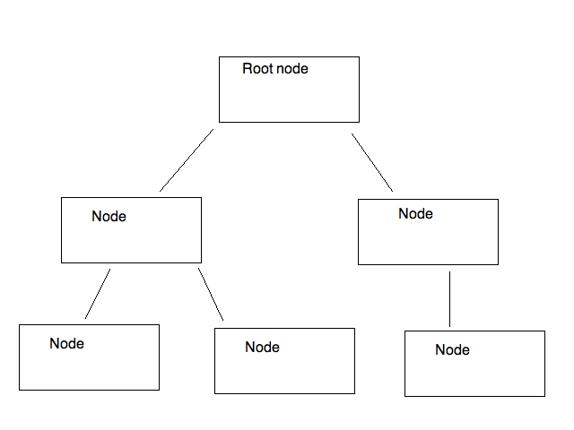
A tree is a commonly-used data structure to represent data in a hierarchical manner. An example of a tree is shown below:

As can be seen, a tree structure resembles a real tree, but is upturned. It consists of a series of nodes, and each node can have one or more descendants. We can easily perform an operation on each node of the tree by starting at the root node, then looping through each immediate descendant in turn. Within a descendant, we loop through its descendants, and so on.

What are trees used for?

Trees have a variety of uses in computing, including:

• Representing directory (folder) structures. The top-level directory is the root of the tree, and its sub-directories its descendants.
• Representing hierarchical documents, such as HTML, the language of web pages. In HTML pages, the page contains a body (the content), the body can contain sections, and sections can contain paragraphs and images. Thus the body can be seen as the root node, a section would be the descendant of the body, and a paragraph or image, a descendant of a section.
• Providing a way of sorting and searching for data efficiently - we will see this during this week and subsequent weeks in the algorithms section of the module.
• Scene graphs in graphical applications such as games. A scene graph is a way of organising 3D components of a graphical application so that 3D objects can have child, or descendant objects - and that any transformations applied to the parent object will be applied to all its descendants. For example a horse object might have a rider object. The rider would be a descendant of the horse. When the horse moves or turns, we want the rider to move or turn with it.

Binary Trees

A binary tree is a form of tree in which each node has two child nodes, a "left node" and a "right node".

This structure can be used to sort data. If you have an array of sortable data, such as numbers or words, you place the first member of the array inside the root node (the top node of the tree). With each subsequent item of data, you place the item in the left node if the data item is less than the item in the root node, and in the right node if the data item is greater than the item in the root node. If the appropriate child node is already filled with data, we descend the tree by moving down to that child node, and then comparing the new value to the value in the child node and then placing it in either the left or the right child node of that node.

This is probably best illustrated by example. Imagine you want to sort the numbers 29, 20, 17, 40, 25, 18, 1. How might you do that with a binary tree?

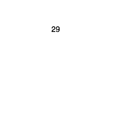
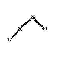
You put the first number (i.e. 29) in the root node of the tree:

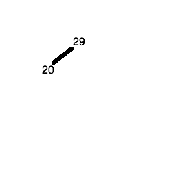
The next number (20) is less than 29, so it gets placed in the left child node of the tree:

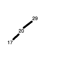
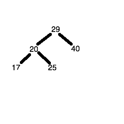
The third number (17) is less than 29 and less than 20, so first we descend the left node of the root node (containing 29) and reach the node containing 20. 17 is less than 20 as well, so it gets placed in the left child node of the node containing 20.

The fourth number (40) is greater than 29, so it gets placed in the right child node of the root node.

The fifth number (25) is less than 29 but greater than 20, so first we descend the left node of the node containing 29, to reach the node containing 20. Since 25 is greater than 20, we place it in the right child node of the node containing 20.

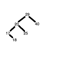
The sixth number (18) is less than 29, so we descend the left node of the root node to get to the node containing the number 20. 18 is less than 20 so we descend the left node again, to reach the node containing the number 17. 18 is greater than 17, so 18 is placed in the right child node of the node containing the number 17.

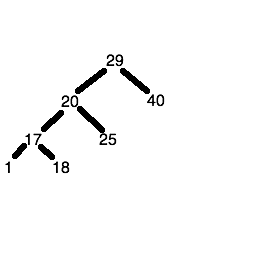
The seventh number (1) is less than 29, so we descend the left node of the root node to get to the node containing the number 20. 1 is less than 20 so we descend the left node again, to reach the node containing the number 17. 1 is less than 17, so 1 is placed in the left child node of the node containing the number 17.

Exercise 1

On paper, create a binary tree containing these numbers in order:

 389 843 9 8934 1 83 23 1124 532

How do we retrieve the sorted data?

Once we have placed the data in the tree, how do we actually retrieve it to display it (or operate it in some other way) in order?

1. Start at the root node.
2. Descend to the left child node.
3. If it has child nodes of its own:
   • first descend its left child node and print out the value within;
   • print out the value within this node;
   • then descend its right child node and print out the value within.
4. If it does not have child nodes of its own, simply display the value within.
5. Repeat the process with the right child node of the root.

What do we do if the left child node's own left child node also has child nodes? We simply repeat the process and keep going until we finally hit a node with no child nodes of its own.

Again this is probably best illustrated by example. Taking the tree produced above:



• The 29 node has two child nodes, 20 and 40, so we descend to 20 first.
• The 20 node has two child nodes, 17 and 25, so we descend to 17 first.
• The 17 node has two child nodes, 1 and 18, so we descend to 1 first.
• 1 has no child nodes, so we just print out 1 and ascend to its parent (the node containing 17)
• Having dealt with the left child of the node containing 17, we print out the value itself (17) first, then descend to the right node (18)
• The 18 node has no child nodes, so we just print out 18
• We then ascend back to the 17 node. The 18 node was the right node of the 17 node, so we are done processing this branch of the tree. So we go back up again to the 20 node.
• We have dealt with the left branch of the 20 node, but not the right. This means we first print out the value, 20 and then descend the right node.
• The right node of 20 contains a value, 25, but no child nodes of its own so we just print out the value (25)
• We then ascend back to the parent, 20, as we are done with this branch.
• We have also covered all branches of 20, so we ascend back up to the root node, 29.
• We have dealt with the left branch of the 29 node, but not the right. This means we first print out the value, 29 and then descend the right node.
• The right node of 29 contains a value, 40, but no child nodes of its own so we just print out the value (40)
• We then ascend back to the parent, 29, as we are done with this branch.
• We have now covered the left branch, the value, and the right branch of the root node. This means we are done with the tree. If you track back the order in which the values were printed, you'll find they are in order:

  1 17 18 20 25 29 40

Recursion

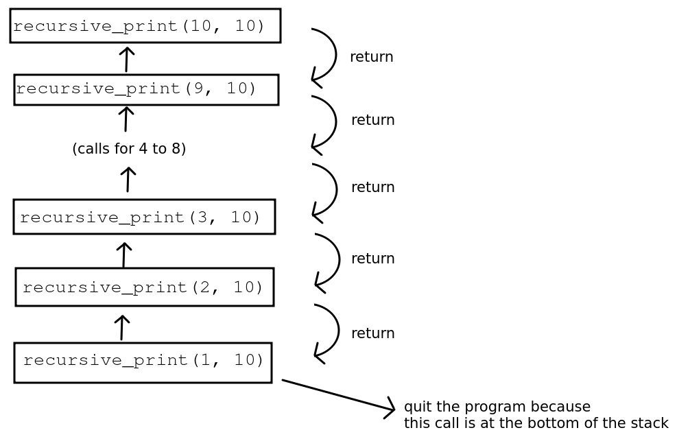
To implement a tree effectively we have to use a programming technique called recursion. The idea of recursion is that a function calls itself repeatedly until some condition is met. You can think of this as producing a stack of calls to the same function, one on top of each other. Then we stop recursing and descend the stack of function calls. To illustrate the concept here is some code to print out the numbers 1 to 10 using recursion:

def recursive_print(num, limit):
    print(f"    recursive_print(): parameters: num {num} limit {limit}")

    if num <= limit:
        print(f"Number is {num}")
        print(f"    num does not exceed {limit}, so calling recursive_print again with argument of {num+1}")
        recursive_print(num+1, limit)

    print(f"    Returning from recursive_print call which has a parameter of {num}")

recursive_print (1, 10)

• We call the recursive_print function with the arguments 1 (representing the current value) and 10 (the maximum value).
• The function prints the current value (1) and then compares the current value (1) to the maximum value (10). Because the current value is less than the maximum, the if statement runs, which adds one to the value (so it becomes 2) and then calls the function again. This is the recursion.
• The function then runs again. 2 is still less than 10, so we print out the value 2, add one to the value (to give 3) and call the function yet again.
• Eventually the current value will become 10. At this point, we print out the value (10) but the if statement will no longer whole true, because 10 is not less than 10. So the call to recursive_print() with the value parameter equal to 10 will immediately return.
• This then returns us to the call to recursive_print() with the value parameter set to 9. Since there are no more statements in recursive_print() after the call to itself, this call also returns immediately.
• We then return to the call to recursive_print() with the value parameter set to 8, which also immediately returns and so we keep descending the stack of function calls until we return to the original call, where value was 1.
• We then return to the main program (outside the function) and our program exits, having printed 1 to 10 in order recursively.

Here is a diagram showing this example of recursion.

Using recursion on a binary tree

So how would we use recursion on a binary tree?

• Start at the root node and:
  • Descend the left branch (see below);
  • Print the value in the node.
  • Descend the right branch (see below)
• For each node we get to (for example the immediate child nodes of the root node), perform the first three steps again:
  • Descend the left branch, if it exists
  • Print the value in the node.
  • Descend the right branch, if it exists
• Hopefully you can see that the act of descending a branch is recursive, because when we descend a branch to reach a child node, we then may need to descend a branch again. Once we get to the bottom of a tree, we then ascend the tree again by returning from each successive function call.

Example of tree recursion from the Python standard library

The walk() function from the os module allows you to "walk" a directory tree (note: not a binary tree) structure, starting at the root directory and recursively descending into subdirectories. For example:

import os

# walk the "src" directory and all its subdirectories
for directory in os.walk("src"):
    print(directory)

Exercise 2: Creating a Binary Tree and using it to sort some data

1. Create a TreeNode data structure to represent a single node in a tree:

   class TreeNode:
       def __init__(self, value):
           self.left = None
           self.value = value
           self.right = None
   

2. Create a BinaryTree class with one attribute, root (the root node of the tree) and two methods: insertNode(), which adds a value to the tree, and printFrom(), which prints out a part of the tree starting at a given node. These two methods should initially be blank (e.g. containing just pass).
3. Implement the insertNode() method in BinaryTree. This should take one parameter: the value to insert, and do the following:
   • If the root node already exists, insert the value into the root node by calling the root node's setChild() method, see below. This will recursively search the tree for an appropriate node to add the value, as discussed above.
   • If it doesn't exist, create the root node and set the root node's value to the value passed in.
4. Write an setChild() method in the TreeNode class. This should:
   • See if the value is less than or greater than the current node's value;
   • If the value is less than the current value, see if there is a left child node. If there is not one (i.e. it's None), create a node storing the value passed in. If there is a left child node, then we'll have to pass the value onto it. So, recursively call the setChild() method on the left node. The effect of this will be to search the tree to find a suitable node to insert the value.
   • If the value is greater than the current value, do the same but with the right node.
5. Implement a printFrom() method in BinaryTree. This should take a parameter which represents the node to start printing from, initially the root node.
   • Declare a variable which represents the current node. Set this initially to the root node.
   • Recursively call printFrom() on the left node, if the left node exists (i.e. is not None)
   • Print the value in the node.
   • Recursively call printFrom() on the right node, if the right node exists (i.e. is not None)
   This will print the whole tree, and nicely illustrates the power of recursion!

Tree searching

We can efficiently search a tree by virtue of its structure. There are two general techniques for searching a tree:

• Depth-first search. This uses the recursive tree traversal technique we have examined already above, starting at the root node and then recursively descending into the child nodes. When the search term is found, we will return it. If the tree is not sorted, we need to keep track of which nodes have been visited and which have not, so we can explore the whole tree.

• Breadth-first search. Rather than recursively descending the tree, we instead we consider each level one at a time. So if we have a tree organised as below:

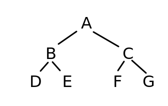
we would first consider node A (the first level), then nodes B and C (the second level), then nodes D, E, F and G (the third level).

Binary search tree (depth-first)

This uses the technique we have seen already to search a tree for a given key (index), namely recursion. We recursively search each successive child node, starting at the root node, until we find the key we are looking for.

For the search to be efficient, we need the tree to be sorted. We have seen already how to add items to a tree in sorted order. The search technique can be considered a specific case of depth-first search in which the tree is sorted and thus we know whether to select the left or right child node, and can ignore the other. For general depth-first search, we cannot guarantee this, and we will need to "backtrack" along branches of the tree to ensure all nodes are visited. In fact depth-first search is a general technique that works on graphs - to be covered later - as well as trees. As we will see, graphs are usually not sorted in any way.

To search a sorted binary tree we need to:

• Start at the root node and test that first. Return the value if the key matches.
• If the root node key is less than the key we are searching for, descend to the right node, otherwise descend to the left node.
• Repeat the process recursively until the key matches; when that happens, return the value.

Hopefully you can see that the complexity is of O(log n) form and it scales well to large values of n, the number of items stored in the tree.

• If the tree has one level (a root only), we search one node.
• If the tree has two levels (three members), we search two nodes.
• If the tree has three levels (seven members), we search three nodes.
• If the tree has four levels (15 members), we search four nodes.

The table below shows the relation between the number of nodes in a sorted and balanced binary tree, and the number of searches. (A balanced tree is one in which the data is evenly added to the left and right sides of the tree. There are techniques for ensuring this, but we will not have time to cover these in this module; I will leave this up to you to research).

Breadth-first search

This section covers breadth-first search in some detail. It is of note that breadth-first search does not require recursion.

Note the order again in which we consider our nodes: A (the root node) first, followed by B and C (the root's child nodes), followed by D, E, F, and G (the child nodes of B and C).

Our aim is to try and search for a value in the tree. How might we do this? We check A first, adding it to a collection of nodes to be considered.

[A]

If A doesn't match, we move on to its child nodes - B and C - and remove A from the collection of nodes to be considered. So, once we've considered and rejected A, the collection will contain B and C.

[B C]

If B doesn't match, then we know we might need to consider its child nodes (D and E) so we add them to the collection of nodes. Because we are doing a breadth first search, though, and considering the tree "level by level", D and E must be added to the collection of nodes to be searched after C - because when we consider B, we will not have considered C yet, and C is on the same level as B. So after considering B, we remove it fron the collection of nodes to be considered - so we are left with:

[C D E]

Next we consider C. If C doesn't match, then we know we might need to consider its child nodes (F and G) so we add them to the collection of nodes to be considered. Because we consider each level left-to-right, these should again be added to the collection after D and E. If C doesn't match, again we remove it, so at this stage, the collection of nodes to be considered will be:

[ D E F G ]

Hopefully you can see that it has linear O(n) complexity, dependent on the number of nodes, and thus is not especially efficient when it comes to simple trees. The use of breadth-first search becomes more apparent when we look at graphs; I am introducing the algorithm here so that you understand it when we begin the graphs topic.

Which data structure to use for the nodes to be processed?

We use a queue here, because with the breadth-first search, we process the nodes in the order they are added. In other words, the node we add first is the node we process first. We can use the standard library collection collections.deque to do this. A deque is a double-ended queue: a queue which you can add to and remove from both the front and back of. However, here we are just using it as a regular queue.

Here is an example of using a deque as a regular queue. Note how we use append() to add to the deque, and popleft() to remove from it.

import collections

q = collections.deque([])
q.append(123)
q.append(456)
q.append(789)
print(q.popleft())
print(len(q))

Using trees to store key/value pairs

I have said several times that we test whether each node 'matches'. What exactly do we mean by this? We'd typically use a tree to store and efficiently search for data as an alternative to hash tables. In other words, each node would contain a key/value pair, such as "1smitj01"/"John Smith" for the key and value respectively in a student records system. In Python, this would probably be stored as a tuple (if we didn't want to change the values) or two-member list (if we did). So we could search the tree for a given key (index), and test each node we find in breadth-first (or depth-first) search to see if its key is the key we are searching for. If it is, then we return the value.

Exercise 3

Start with your own tree from above.

1. Implement either depth-first or breadth-first search using the tree (for now return True or False depending on whether the number is in the tree or not).
2. If you finish question 1, implement the other search.