We are now going to start looking at algorithms. An algorithm is, as we have seen, a clearly-defined solution to a particular problem, which follows a series of clearly-specified steps. Common examples of algorithms include sorting collections of data, or searching for an item in a collection of data.
We will start by looking at algorithm efficiency using the Big O notation, and then look at some sorting and searching algorithms, comparing their efficiency.
When designing algorithms, we need some measure of how complex an
algorithm is. Complexity can be measured in various ways, for example
performance (time taken), or memory usage. The standard for measuring
algorithm complexity is known as the Big O notation. This is a measure
which expresses complexity in relation to some property n. This property
depends on exactly what we are trying to do. For a sorting algorithm, which
sorts a list, for example, it could be the number of items in the list. For
indexing a list or linked list, it could also be the number of items in the list; the larger the list, the more items we potentially have to traverse to reach a given index.
"Big O" notation is expressed in terms of this property n. For example
we can have:
O(1) : if an algorithm is O(1) it means that its complexity is independent of n. Calculating the memory address of the index of an array would be an example of an O(1) operation because it is always given by the equation:memory_address = start_memory_address + index * bytes_used_by_one_item
Clearly the time taken to evaluate this equation does not depend on the
size of the list, which is the property n in this case. Even if the list is very large, and the index is very large, we can quickly calculate the item's address using the simple equation above. O(1) algorithms are thus highly efficient… but not many algorithms are O(1)!
O(n) : if an algorithm is O(n) it means that its complexity depends on
the value of n directly, or linearly.
So if n increases by 2, the complexity will also
increase by 2 Indexing a linked list is a good example of an O(n)
algorithm because we have to manually follow the links to retrieve the item
with a given index - we cannot rely on consecutive memory addresses. So
complexity of linked list indexing is related linearly to the length of the
list.This brings up an important point, the big O notation used is the worst-case scenario. In a basic search such as this, we assume the index will not be found until the end of the list in which case we will have to search through n items, where n is the number of items in the list.
A basic search for an item in a list, in which we loop through all members of the list until we find the search term we are looking for, is also O(n): it's again linearly related to the length of the list, because in a worst-case scenario, we will have to search through the entire list before we find the item.
O(n^2) (^ indicates "power"): if an algorithm is O(n^2) then the time taken or memory used is most influenced by the square of the number of items. So if the number of items doubles, then the time taken will increase around four times. Or if the
number of items increases by 10, the time taken will increase around 100 times.Algorithms which have an outer and inner loop, in which we have to loop through an array twice, are of this kind. The outer loop has to be run n times,
but the inner loop has to be run n times each time the outer loop runs.
So the time taken is proportional to n^2. For example, below is some code
with two loops, an outer and inner loop. An algorithm do_something() is
performed n^2 times (16 times in the example, as n is 4). If n is changed
to 5, then the operation will be performed 25 (5^2) times.
n = 4
for i in range (n):
    for j in range (n):
        do_something(i, j)
Clearly it can be seen that O(n^2) algorithms are not efficient, and should
be refactored to a more efficient algorithm e.g. O(n) or, as described
below, O(log n).
O(n^2) algorithms are known as quadratic because their complexity can be calculated using a quadratic equation an^2 + bn + c. It should be noted that,
depending on the exact algorithm, the complexity will not be exactly
n^2. However it will be something close to n^2 which can be expressed
using a quadratic equation. If you consider a quadratic equation, it can be
seen that, as the variable n increases, the n^2 term will come to
dominate the result.
3n^2 + 6n + 7
for the value n=100 will be:
3(100^2) + 6(100) + 7
which is
30000 + 600 + 7
It can be seen that the n^2 term dominates. Remember we said above that
in Big O notation, we need to worry about worst-case scenarios (scenarios with
large n typically) as these will be the main source of inefficiencies.
So it can be seen that, in these worst-case scenarios, even if the complexity
is not exactly n^2, it will approximate to it. So, such algorithms are still designated O(n^2).
Essentially, when considering complexity with the Big O notation, we divide algorithms into classes, and ask ourselves which class (e.g. O(1), O(n), O(n^2) etc) does the algorithm fall into, depending on the behaviour of the algorithm
for large n. We are less interested in an absolute value for the time taken, or memory used, to complete an algorithm and more interested in the algorithm's behaviour for very large values of n, so we can see what happens in worst-case scenarios.
The diagram below shows how complexity increases with increasing n for
different classes of Big O complexity:
n is along the x (horizontal) axis, while the complexity is along the y (vertical) axis;O(n);O(n^2);O(log n); to be discussed below;0.5*n^2 + 0.5n. This shows that the quadratic form is exhibited, and the shape of the graph, with a rapid increase with the rate of increase getting bigger with larger values of n is very similar to n^2. (This is known as a parabolic graph). So, even if the complexity is not exactly O(n^2), the behaviour of the graph for increasing n is essentially the same as O(n^2).O(log n): if an algorithm ia O(log n) it is related to the logarithm
of n. Logarithm is the inverse operation to power, and is always expressed in
terms of a particular base. A logarithm of a given number (relative to a particular base, such as base 10 or base 2) will give you the power the base has to be raised to, to give that number. So if b to the power p equals x, then log(b)x = p.b^p = x => log(b) x = p
In Big O notation, the base is 2. So for example, if:
2^2 = 4
2^3 = 8
so:
log(2) 4 = 2
log(2) 8 = 3
Hopefully you can see from this that an O(log n) operation is relatively
efficient, because we can increase n significantly but the time taken, or
memory consumed, will increase much less. For example, to perform an
O(log n) operation on a list of 256 (2^8) items will only take twice as long as a list of 16 (2^4) items. Constrast that to an O(n) algorithm which will take 16 times as long (because 16 x 16 is 256). So if you can refactor an algorithm from O(n) to O(log n), it is clearly desirable.
You should be able to see that an O(log n) operation has an initial fast increase in complexity which then flattens out. Algorithms which involve one complex operation which must be done once, or a small number of times, no matter what the value of n, followed by a less-complex operation, will typically be of the form O(log n).
We are now going to start looking at sorting algorithms, and consider the Big O complexity of each algorithm we examine.
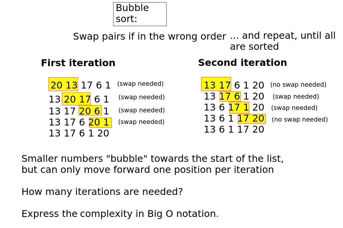
We are now going to look at various sorting algorithms and express their complexity in Big O notation. The first algorithm we will look at is the bubble sort. This is a simple algorithm, but it is not very efficient. As you can see from the diagram below, it involves looping through a list and considering each pair of values in turn. If the pair is in the correct order, we do nothing. If it is not, we swap them.
As you can see from the diagram, larger numbers "bubble" towards the end of the list, for example the value 20 will, each time a swap is done, move one position onwards in the list. So once we've finished the first iteration of the sort, the largest value will be in the correct position. However, you should also be able to see from the diagram, and appreciate from the way the algorithm works, that the smaller values only move forward one position per iteration (i.e. one position per loop). So once we've finished the loop, the value 1 will only have moved forward one place.
So we then need to iterate (loop) again through the list, and perform another series of swapping operations. You can see this on the "second iteration" part of the diagram. This results in the smaller numbers again moving forward just one position.
We'd therefore need to implement this using a loop within a loop. The outer loop would be the successive iterations, whereas the inner loop would be used to perform the swapping operations of one particular iteration of the algorithm.
It should be noted that on the first iteration of the bubble sort, the largest value will be correctly in place at the end of the list. So on the second iteration, we do not need to consider the last position in the index; for example if there are 5 values, we only need to consider 4 in the second iteration. Similarly, at the end of the second iteration, the second-biggst value will be correctly placed, so on the third iteration we do not need to consider the final two values of the list.
Bubble sort (and many other sorts) require variables to be swapped. How can we do this? We would use code such as this, involving the creation of a temporary variable.
tempVar = a
a = b
b = tempVar
We cannot just do:
a = b
b = a
because the first statement will set a to b before we've saved the value
of a anywhere else, so when we execute the statement b = a we will set
b to its original value, because we a now contains the value of b.
The use of a temporary variable, as in the correct example, means we can
store a before assigning the variable a to the value of b, which means
we do not lose the original value of a.
However, in Python there is a shortcut for swapping variables which does this for us:
a,b = b,a
On paper, continue the iterations of bubble sort to sort the values. After how many iterations are the values completely sorted?
How could we express the time taken in terms of n, i.e. the number of items
in the list?
What, therefore, would be the complexity in Big O notation of this algorithm, where n is the number of values in the list?
Have a go at coding bubble sort in Python. You should create a list of numbers to sort, and once the algorithm has finished, print the list to test whether the sort has taken place. If you are struggling, try writing it in pseudocode first.
Selection sort is another sorting algorithm which is conceptually simple but (relatively) inefficient. Nonetheless it has some advantages over bubble sort,
in particular, the number of swap operations is minimised (of order O(n) rather than O(n^2)), and will be used as another example of a sorting algorithm.
We once again have an outer loop. This loops through each member of the list (apart from the last). Within the outer loop we have an inner loop which compares the current member with each of the remaining members in turn. The lowest remaining member is found, and if this is lower than the current member, the current member and this lowest member is swapped.
See the diagram below, which is based from notes provided by my former colleague Brian Dupée, which were in turn sourced from the site sorting-algorithms.com (this site still exists, provided by Toptal, but does not appear to contain these resources anymore)
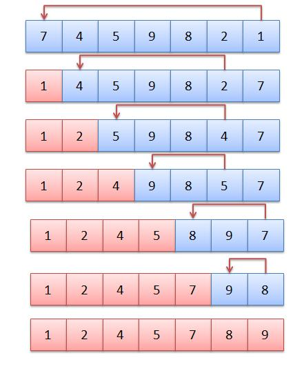
It is of interest what this algorithm's time complexity equals, as it raises an important conceptual point about the Big O notation. If you imagine sorting 5 values, what needs to be done?
n-1, or 4 swaps.So the total number of operations for a 5-member list is 4+3+2+1, or more generally for an n-member list, the number of operations is the sum of all the numbers from 1 to n. This value is equal to (n + n^2) / 2.
This is an equation of quadratic form, as it can be expressed instead as 0.5n^2 + 0.5n. So with large n values the n^2 term will dominate, and thus, this is an O(n^2) class of algorithm, i.e. less efficient. It is not quite as inefficient as bubble sort, particularly given that less swaps are involved (swapping is a relatively expensive operation as it requires a temporary variable to be created), but it can still potentially be improved.
A less mathematical way of thinking about it is to consider the fact that there are two loops, one within another. Algorithms of this form - even if one of the loops does not iterate through the entire list - will generally be O(n^2).
When swapping numbers, swapping is not particularly computationally expensive. However, if the two values are complex objects which take time to initialise, then the fact that we need to create a temporary variable can mean a swap is expensive. So in cases like this, selection sort is particularly favoured over bubble sort.
Have a go at implementing selection sort in Python.
As we saw above, searching through a list is an O(n) operation, as the worst-case scenario performance will be linearly proportional to the length of the list. We have to loop through each member of the list until we find the item that we are looking for, which, if near the end of the list, may take some time.
This approach is known as brute-force. Brute-force algorithms attempt to find an answer through testing every possibility (here, every item in the list) and do not try to use any optimisations or more efficient techniques. Another example of a brute-force algorithm would be trying to find the factors of a number (factors of a number are every integer that the number can be divided by to give a further integer, for example the factors of 24 are 2, 3, 4, 6, 8 and 12). What we could do in a brute-force algorithm is to divide the number by every integer from 2 to the number to see if we get an integer as a result. This works, but is not efficient (O(n) with respect to the number).
Another perhaps notorious brute-force technique is one which, sadly, has been proven successful despite the time taken, and that is brute-force password attacks. In this, every possible password of a certain length is tested on a login system. The result will be that the password will eventually discovered. Brute-force password attacks are now feasible due to increased computing power, notably brute-force dictionary attacks (in which known words are tested) which is the reason why longer and more obscure passwords - with special characters, lower- and upper-case letters, and numbers - are now recommended compared to say 20 years ago.
Binary search is a significantly more efficient approach to searching than ordinary brute-force search (called linear search). It has O(log n) complexity, which as we saw last week, will mean it performs much better with large sets of data than an O(n) algorithm.
How does binary search work? It works by repeatedly "guessing" a position to index in a list to find a particular item of data. This is described in more detail below, but one point that needs to be made clear is that the data should be sorted - using a sorting algorithm - first. You might be asking yourself, wouldn't that make binary search not particularly efficient compared to linear search, as we have to sort first? The answer is - not necessarily. In many use-cases, such as, for example, searching for a record in a large list of people in some sort of records system (such as a student records system) it's likely that searching will have to be done many, many times. By contrast, the data would only have to be sorted once - i.e. when the data is first created - or at worst, when a new record is added to the data, which is likely to be infrequent.
Binary search is known as a divide and conquer algorithm because the data we are searching is repeatedly divided in order to efficiently find what we are looking for. This is how you would play a "guess the number" game. Someone would try to repeatedly guess a number, and the other person would say "lower" or "higher". The person guessing would then use the other person's response to narrow down the range of numbers they select from.
Here is an example of binary search. We have an array with 100 members containing names sorted in alphabetical order, and we are searching for "Smith, Tim".
math.floor((start + end) / 2) # need to import math
where start is the start of the portion of the list we are searching (0 - as
we are searching the whole list) and end is the end of the portion of the list
(99 here, assuming a list of 100)
then it will always give a suitable midpoint to index. Note that math.floor takes a floating-point number and rounds it down. If the length is an even number (e.g. 100) it will give us the index of the item immediately before the midpoint (49) while if it is an odd number (e.g. 101) it will give us the exact midpoint (because indices start from 0 and math.floor(101/2) is math.floor(50.5) which is 50, in other words, exactly halfway between 0 and 100.
So, say we find "Jones, Jane" at position 49 in our example. We know we need to look within the range 50-99 because "Smith, Tim" is after "Jones, Jane" in the alphabet.
So we repeat the divide-and-conquer operation. We find the midpoint of 50 and 99 (74) and look at the value there. It's "Nodd, Nigel".
We repeat the process. "Smith, Tim" is after "Nodd, Nigel" in the alphabet so we know we have to search the portion of the list after 74. So we find the midpoint of 75 and 99, which is 87. We might get "Trott, Tina" at this position, so now we need to look at the portion before 87 (as "Smith, Tim" is before "Trott, Tina" in the alphabet). So we have to search within the portion75-86. We choose the midpoint, 80, and now found "Raven, Roger".
Our area of search is cut down now to 81-86. We pick 83 and find "Smith, Alice", i.e just before "Smith, Tim" alphabetically. We then only have three list positions to search - 84 to 86. So we pick the midpoint 85. We find "Smith, Simon". We now only have one possibility - 86 - and looking at item 86 we finally find what we want, "Smith, Tim".
The diagram below shows the process. Our search term (Smith, Tim) is shown using a red circle.
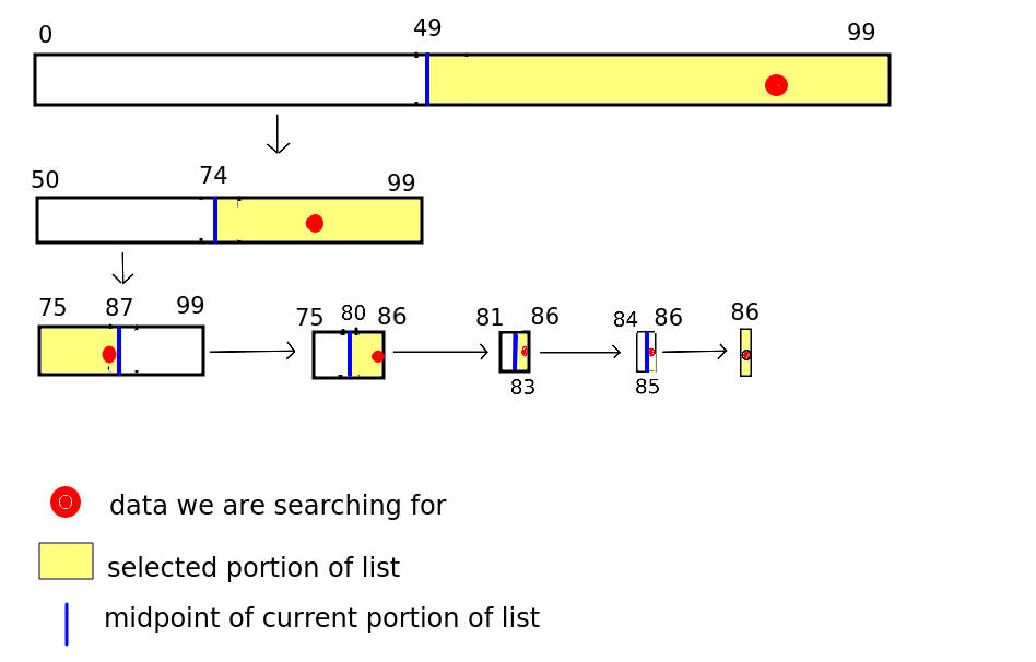
So how many searches did we need until we found Smith, Tim?
Clearly 7 checked items (and this was a worst case scenario here, as we only found what we were looking for after narrowing down the possibilities to one) is a good deal more efficient than the 87 we would have to check with a brute-force linear search!
O(log n)?The complexity of binary search is O(log n), with n the number of items in the list. In our example n was 100. What is log(2) 100? The exact value does not matter, but we know it will be between 6 and 7, as log(2) 64 is 6 and log(2) 128 is 7. So you can see that O(log n) fairly represents the complexity, as, in this worst-case scenario, we had 7 iterations.
How can we prove this? Think of a list with an exact power of 2 length, such as 64, and imagine it's a worst-case scenario, where we have to narrow down to one possibility before we find what we are looking for.
So the length of the portion under search decreases from 64-32-16-8-4-2-1 in each iteration of the list. In other words, assuming the list length is an exact power of two, the number of iterations will be log n + 1 (+1 because we also check a list of length 1 as well as the various powers of two; the lengths in each subsequent iteration are 2^6, 2^5, 2^4, 2^3, 2^2, 2^1 and 2^0 - i.e. 1). But as we saw last week, we only need to take the most significant term of the complexity and can discard the +1 (as we are interested in the general behaviour of algorithms at large n, not the exact complexity) - giving us O(log n).
Likewise, for a value n between 2^p and 2^(p+1), the number of iterations will be p-1, or log(floor(n))-1 - but again we can simplify to O(log n). (For example, try repeating the above on a list of length 63, a value between 32 and 64, and you find that only six iterations are needed, as the length of the portion being searched will decrease 63-31-15-7-3-1).
while loop. What condition, involving the variables in question 1, will be true when the binary search ends? This condition should be used in your while loop.